光学薄膜特性理论计算1-菲涅尔公式

摘要

光在界面的传播是薄膜理论的基础，本文从麦克斯韦方程组出发推导菲涅尔公式。

1.折射率与光学导纳^[1]

麦克斯韦方程组如下

\[ \begin{align} % Gauss's law for electricity \nabla \cdot \mathbf{D} &= \rho \nonumber \\ % Gauss's law for magnetism \nabla \cdot \mathbf{B} &= 0 \nonumber\\ % Faraday's law of electromagnetic induction \nabla \times \mathbf{E} &= -\frac{\partial \mathbf{B}}{\partial t} \nonumber\\ % Ampère's circuital law with Maxwell's addition \nabla \times \mathbf{H} &= \mathbf{J} + \frac{\partial \mathbf{D}}{\partial t} \nonumber \end{align} \]

将\(D = \varepsilon E\) , \(J = \sigma E\)代入麦克斯韦方程组的安培环路定律可得

\[ \nabla \times H = \varepsilon \frac{\partial E}{\partial t} + \sigma E \tag{1-1} \]

对法拉第电感定律两边取旋度并代入(1-1)有

\[ \nabla \times \nabla \times E = - \mu \frac{\partial (\nabla \times H)}{\partial t} = - \mu \frac{\partial }{\partial t}(\varepsilon \frac{\partial E}{\partial t} + \sigma E \tag{1-2}) \]

运用矢量恒等式\(\nabla \times \nabla \times E = \nabla (\nabla\cdot E)-\nabla^2E\)在无电荷的均匀空间（根据高斯定理\(\nabla \cdot \mathbf{D} = 0\)），上式可以化简为

\[ \nabla^2E = \mu \varepsilon \frac{\partial^2 E}{\partial^2 t} + \mu \sigma \frac{\partial E}{\partial t} \tag{1-3} \]

如果介质不导电，即\(\sigma=0\)，式(1-3)变为

\[ \nabla^2E = \mu \varepsilon \frac{\partial^2 E}{\partial^2 t} \tag{1-4} \]

通过求解微分方程，在不导电的均匀介质中，沿x正方向行进的电磁波的表达式可以写成

\[ E = E_0 \exp[i\omega (t-\frac{x}{v})]\tag{1-5} \]

其中\(v=1/\sqrt{\mu \varepsilon}\)是在介质中的传播速度，\(\omega\)是角频率。电池波在真空中传播的速度和在不导电均匀介质中的速度比值，被称为介质的折射率，公式如下：

\[ n = \frac{c}{v}=\frac{\sqrt{\varepsilon \mu}}{\sqrt{\varepsilon_0 \mu_0}} = \sqrt{\varepsilon_r \mu_r}\tag{1-6} \]

在光频率下，光学材料的磁导率可以近似认为是1，所以有\(n=\sqrt{\varepsilon_r}\)

式(1-5)可以被认为是式(1-3)的一个特解，对于金属介质（\(\sigma \ne 0\)）,将(1-5)回代，得到

\[ \frac{1}{v^2} = \varepsilon \mu - i\frac{\sigma \mu }{\omega} \tag{1-7} \]

则对于金属介质的折射率有

\[ N^2 = \frac{c^2}{v^2} = (\varepsilon \mu - i\frac{\sigma \mu }{\omega})/\varepsilon_0 \mu_0 \tag{1-8} \]

可知金属的折射率为复数，记作\(N = n - ik\)，回代入式(1-5)得

\[ E = E_0 \exp{(-\frac{2\pi k x}{\lambda })}\exp{ \left [ i(\omega t - \frac{2\pi n x}{\lambda}) \right ] } \]

说明对于金属折射率的虚部会让电磁波发生指数级衰减，所以k又被称为吸收系数。

同理，磁场也可以写做波函数的形式，磁场和电场的表达式如下：

\[ \mathbf{H} = H_0 \exp{ \left [ i(\omega t - \frac{2\pi N }{\lambda}) \mathbf{S_0} \cdot \mathbf{r} \right ] } \]

\[ \mathbf{E} = E_0 \exp{ \left [ i(\omega t - \frac{2\pi N }{\lambda}) \mathbf{S_0} \cdot \mathbf{r} \right ] } \]

其中\(\mathbf{S_0}\)是平面波传播方向的单位矢量，\(\mathbf{r}\)是坐标矢径。

对于\(\nabla \times H = -i\frac{2\pi N}{\lambda}(\mathbf{S_0} \times \mathbf{H})\)带入麦克斯韦方程组得

\[ \mathbf{S_0} \times \mathbf{H} = -\frac{N\sqrt{\varepsilon _0/\mu_0} }{\mu_r} \mathbf{E} \]

\[ \frac{N\sqrt{\varepsilon _0/\mu_0} }{\mu_r} \mathbf{S_0} \times \mathbf{E} = \mathbf{H} \]

上两式说明，电场和磁场是相互垂直的，而且都与传播方向垂直，且符合右手螺旋法则。对于传播过程中，E和H不但相互垂直，且数值间也存在一定比值。

\[ Y = \frac{\left | \mathbf{H} \right | }{\left | \mathbf{S_0 \times E} \right | } = \frac{N\sqrt{\varepsilon _0 / \mu_0}}{\mu_r} \]

Y被称为介质的光学导纳，其中磁导率\(\mu_r\)通常接近于1，若以自由空间导纳\(\sqrt{\varepsilon _0 / \mu_0}\)为单位，则光学导纳与折射率相等。

2.折射反射定律

根据电磁场的边界条件在界面处E和H的切向分量是连续的，有

\[ E_t^i + E_t^r = E_t^t \]

\[ H_t^i + H_t^r = H_t^t \]

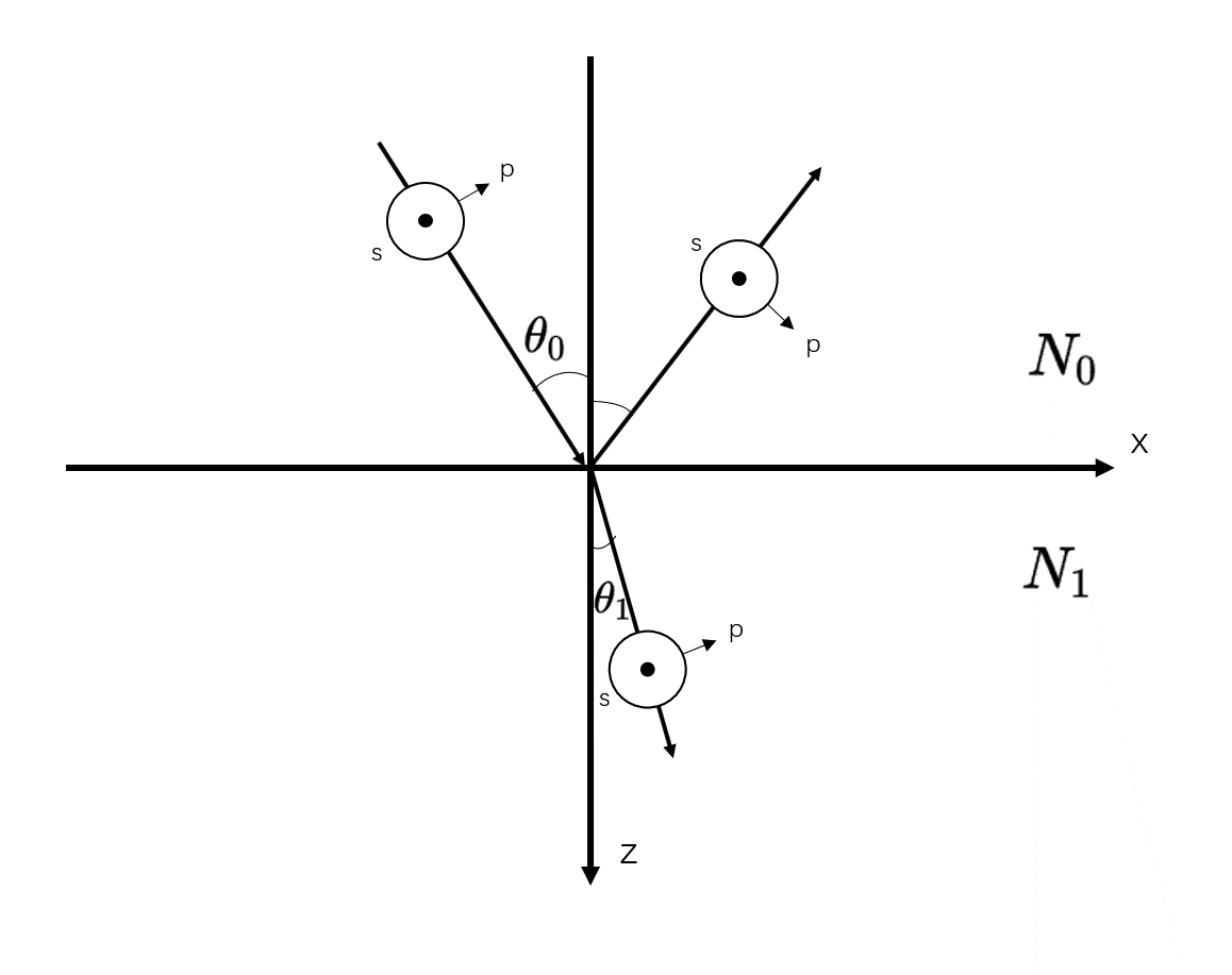
按图中所示，光线在xz平面传播，以\(\theta_0\)的角度入射到界面，界面为\(z=0\)平面。其入射光相位因子为

\[ \exp{\left \{ i\left [ \omega _i t - \frac{2\pi N_0}{\lambda} \left ( \sin\theta_0 x + \cos \theta_0 z\right ) \right ] \right \} } \]

设反射光和透射光的相位分别为

\[ \exp{\left \{ i\left [ \omega _i t - \frac{2\pi N_0}{\lambda} \left ( \alpha_r x +\beta_r y+ \gamma_r z\right ) \right ] \right \} } \]

\[ \exp{\left \{ i\left [ \omega _i t - \frac{2\pi N_1}{\lambda} \left ( \alpha_t x +\beta_t y+ \gamma_t z\right ) \right ] \right \} } \]

要满足边界条件，界面上的相位因子必须相等。所以有\(\beta_r = \beta_t = 0\)、\(N_0 \alpha_i = N_0 \alpha_r = N_1 \alpha_t\)

可以得出反射和折射定律

\[ \theta_0 = \theta_r \]

\[ N_0 \sin \theta_0 = N_1 \sin \theta_t \]

3.菲涅尔公式

3.1 垂直入射情况

为进一步研究反射光和入射光振幅和相位的变化关系，我们先假设光是垂直入射界面的。

对于垂直入射界面的光，显然有E和H都是平行于界面，有 \[ H_1 = H_t , E_1 = E_t \]

又根据边界条件有

\[ E_1 = E_0^+ + E_0^- \]

\[ H_1 = H_0^+ + H_0^- \]

其中下标0和1代表界面的两边，上标+代表正向传播，-代表反向传播。结合上式有

\[ H_1 = N_1(S_0 \times E_1) = N_0(S_0 \times E_0^+ - S_0 \times E^-_0) \]

即

\[ N_1 E_1 = N_0 (E_0^+ - E_0^-) \]

化简可得反射系数和透射系数

\[ r = \frac{E_0^-}{E_0^+} = \frac{N_0-N_1}{N_0+N_1} \]

\[ t = \frac{E_1}{E_0^+} = \frac{2N_0}{N_0 + N_1} \]

3.2 倾斜入射情况

下面考虑倾斜入射的情况。我们将入射的电磁波分解为，电场垂直反射面（s光）和平行反射面（p光）振动的两种状态。

为方便定义切向分量，现引入有效导纳的概念

\[ \eta = H_t^+ / (S_0 \times E_t^+) \]

对于p光（TM波），磁场H垂直于入射面，与界面平行，因此\(H = H_t\)，而电场\(E=Ecos \theta\)

\[ H_t = H = N(S_0 \times E) = N(r_0 \times E_t/cos\theta) = \frac{N}{cos\theta}(r_0 \times E_t) \]

所以对于p光有\(\eta_p = N/cos \theta\),同理对于s光有\(\eta_s = Ncos \theta\)

对菲涅尔反射系数可以写作

\[ r_p = \frac{\eta_{0p}-\eta_{1p}}{\eta_{0p}+\eta_{1p}} = \frac{N_0cos\theta_1 - N_1 cos\theta_0}{N_0cos\theta_1 + N_1 cos\theta_0} \]

\[ r_s = \frac{\eta_{0s}-\eta_{1s}}{\eta_{0s}+\eta_{1s}} = \frac{N_0cos\theta_0 - N_1 cos\theta_1}{N_0cos\theta_0 + N_1 cos\theta_1} \]

对于透射系数可以写作

\[ t_p = \frac{2N_0cos\theta_0}{N_0cos\theta_1+N_1cos\theta_0} \]

\[ t_s = \frac{2N_0cos\theta_0}{N_0cos\theta_0 + N_1cos\theta_1} \]

反射率为

\[ R = r^2 \]

透射率为

\[ T = \frac{N_1cos\theta_1}{N_0cos\theta_0}|t^2| \]

该公式对复折射率介质也同样成立。

给出计算代码如下，其中函数公式中符号相反只影响相位，并不影响透射和反射率。

import matplotlib.pyplot as plt
import numpy as np

def Fresnel(n1, n2, theta1):
    # 角度转弧度
    theta1 = theta1 /180 * np.pi
    costheta1 = np.cos(theta1)
    n1_r = n1.real
    n2_r = n2.real
    costheta2_2 = 1-(n1_r/n2_r*np.sin(theta1))**2
    if costheta2_2 >= 0:
        costheta2 = np.sqrt(costheta2_2)
        rp = (n2*costheta1 - n1*costheta2)/(n2*costheta1 + n1*costheta2)
        rs = (n1*costheta1 - n2*costheta2)/(n1*costheta1 + n2*costheta2)
        tp = (2*n1*costheta1)/(n1*costheta2+n2*costheta1)
        ts = (2*n1*costheta1)/(n1*costheta1+n2*costheta2)    
        temp = n2*costheta2/(n1*costheta1)
    else:
        #发生了全反射
        rp = 1.0
        rs = 1.0
        tp = 0.0
        ts = 0.0
        temp = 0


    return rp**2, rs**2, temp*(tp**2),temp*(ts**2)

theta_ls = np.linspace(0, 90, 100)

N_Bk7 = 1.5214145
N_air = 1

# p光数据
Rp_ls = []
Tp_ls = []
# s光数据
Rs_ls = []
Ts_ls = []
# 平均数据
Avg_r_ls = []
Avg_t_ls = []

# 吸收计算，暂时为 0
absorb = 0

for theta in theta_ls:
    Rp,Rs,Tp,Ts = Fresnel(N_air,N_Bk7,theta)
    Rp_ls.append(Rp)
    Rs_ls.append(Rs)
    Tp_ls.append(Tp)
    Ts_ls.append(Ts)
    Avg_r_ls.append((Rp+Rs)/2)
    Avg_t_ls.append((Tp+Ts)/2)



plt.figure(1)
plt.plot(theta_ls,Rp_ls,color="green",label = 'p')
plt.plot(theta_ls,Rs_ls,color="blue",label = 's')
plt.plot(theta_ls,Avg_r_ls,color="red",label = 'avg')
plt.legend(loc="upper left")
plt.title("R")

plt.figure(2)
plt.plot(theta_ls,Tp_ls,color="green",label = 'p')
plt.plot(theta_ls,Ts_ls,color="blue",label = 's')
plt.plot(theta_ls,Avg_t_ls,color="red",label = 'avg')
plt.legend(loc="upper left")
plt.title("T")
plt.show()

3.3 全反射情况

这里只给出相位公式，公式来着参考资料[1]

\[ \tan \frac{1}{2}\varphi _s = \frac{(\sin^2\theta_0 - n_1^2/n_0^2)^{1/2}}{\cos \theta_0} \]

\[ \tan \frac{1}{2}\varphi _p = \frac{n_1^2/n_0^2 \cdot \cos\theta_0}{(\sin^2\theta_0 - n_1^2/n_0^2)^{1/2}} \]

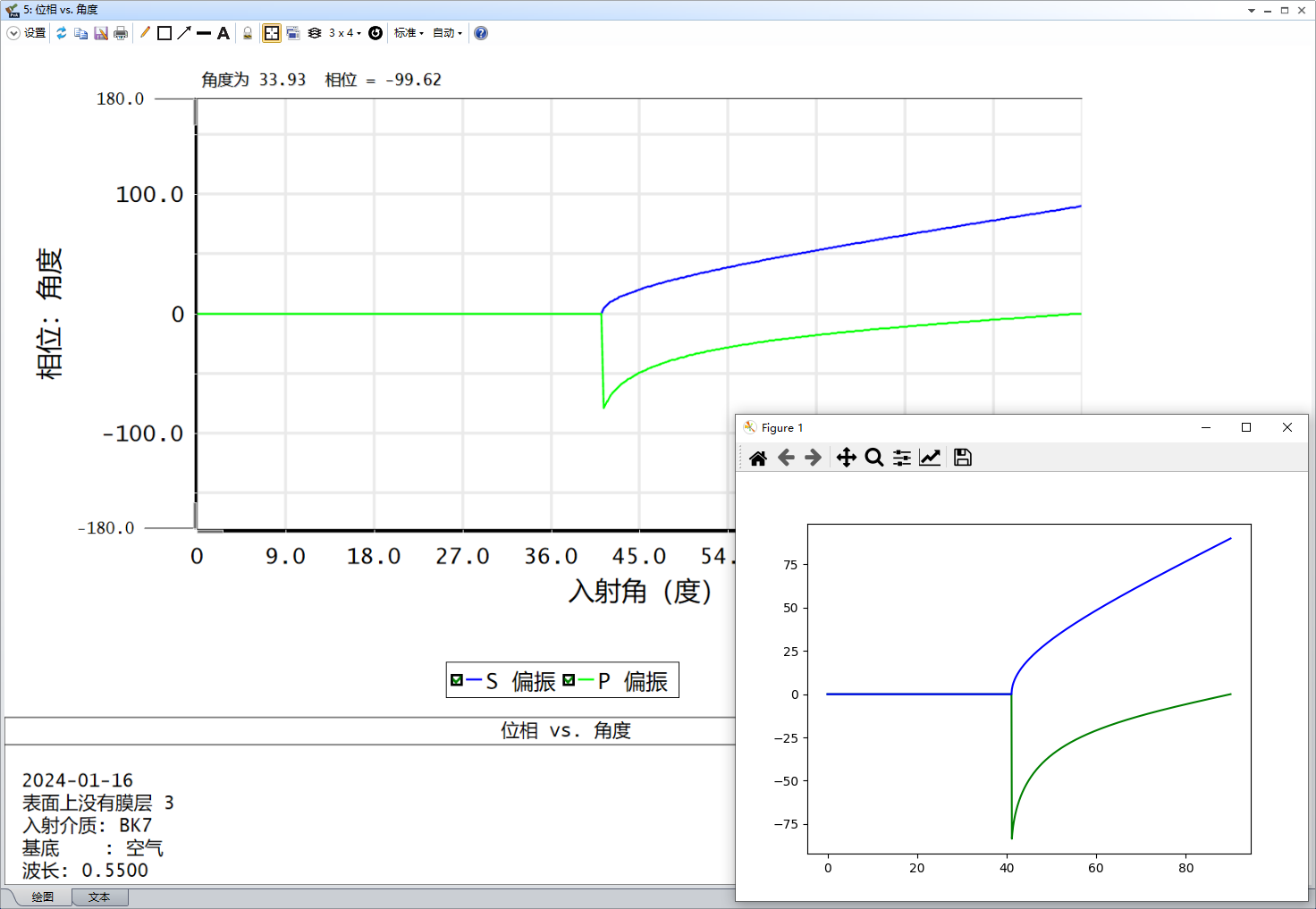
但在使用zemax仿真时，发现相位不需要乘2数值才是匹配的，源码和仿真结果如下

import matplotlib.pyplot as plt
import numpy as np

def Phase(n1, n2, theta1):
    # 角度转弧度
    theta1 = theta1 /180 * np.pi
    costheta1 = np.cos(theta1)
    n1_r = n1.real
    n2_r = n2.real
    costheta2_2 = 1-(n1_r/n2_r*np.sin(theta1))**2
    if costheta2_2 >= 0:
        if n1 > n2:
            return 0,0
    else:
        #全反射
        tande_s = np.sqrt(np.sin(theta1)**2-n2**2/n1**2)/costheta1
        a = (n2**2)/(n1**2) * (costheta1)
        b = np.sqrt(np.sin(theta1)**2 - n2**2/n1**2)
        tande_p = -(a)/(b)
        return np.arctan(tande_p)/np.pi*180,np.arctan(tande_s)/np.pi*180

theta_ls = np.linspace(0, 90, 1000)

N_Bk7 = 1.5214145
N_air = 1

# p光数据
Rp_ls = []
Tp_ls = []
# s光数据
Rs_ls = []
Ts_ls = []


for theta in theta_ls:
    dep,des = Phase(N_Bk7, N_air, theta)
    Rp_ls.append(dep)
    Rs_ls.append(des)

plt.figure(1)
plt.plot(theta_ls,Rp_ls,color="green",label = 'p')
plt.plot(theta_ls,Rs_ls,color="blue",label = 's')
plt.show()

全反射

参考资料

[1] 唐晋发.现代光学薄膜技术.浙江大学出版社.2006年