机器学习实战1
摘要
《机器学习实战:基于Scikit-Learn和TensorFlow》学习笔记
加州房价
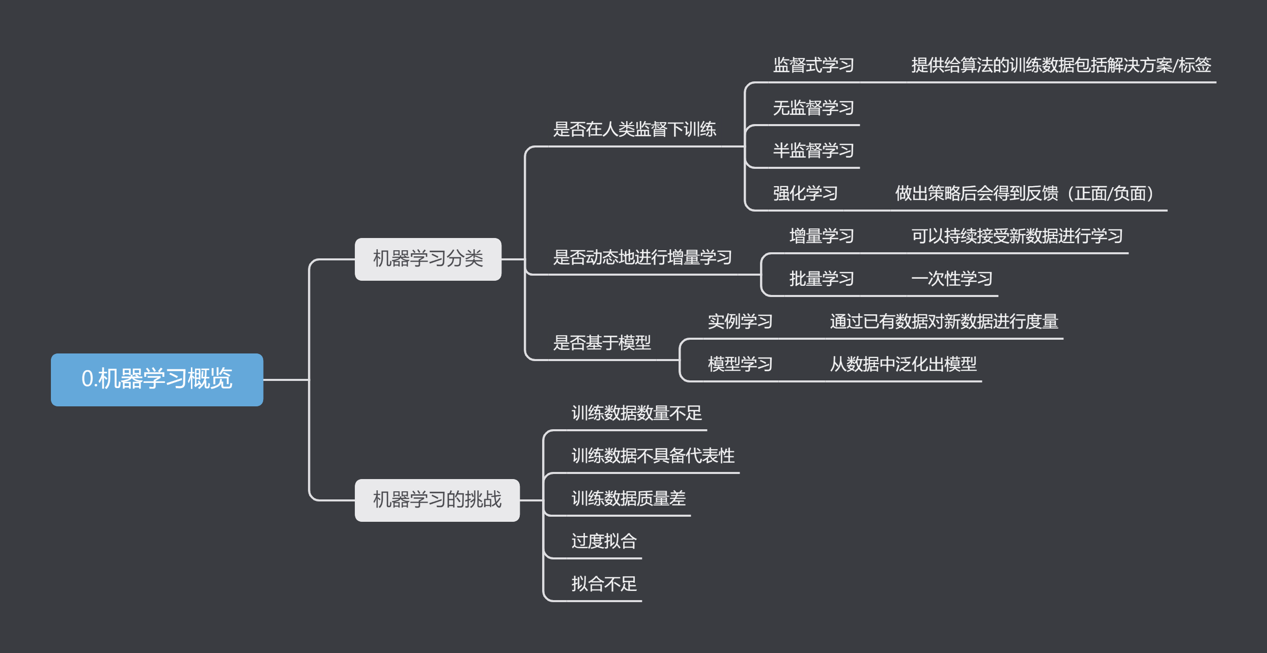
1.机器学习概览
2.机器学习项目--加州房价预测
假设你是一个房地产公司最近新雇佣的数据科学家,你需要根据加州房价数据集建立一个房价模型,使其能预测任意区域的房价中位数。
以下是你可能需要经历的步骤流程
- 观察大局
- 获得数据
- 从数据探索和可视化中获得洞见
- 机器学习算法的数据准备
- 选择和训练模型
- 微调模型
- 展示解决方案
- 启动、监控和维护系统
2.1 观察大局
首先我们需要明确目标,输入和输出是什么?数据是否包含结果?数据是否会更新?
这些问题会决定你的机器学习模型应该是什么样的。输入是人口收入中位数等信息,显然这应该设定为监督式学习,房价数据肯定会更新,但变化不快,批量学习也能接受。
对于房价预测问题,有接触过机器学习的应该都能看出这就是一个典型的多元回归任务。
接下来应该选取一个合适的性能指标,回归问题的典型衡量指标是均方根误差(RMSE),计算公式如下
\[ RMSE(\mathbf{X},h) = \sqrt[]{\frac{1}{m}\sum_{i=1}^{m}(h(\mathbf{x}^{\left ( i \right ) })-y^{(i)} )^2 } \]
其中h()是预测函数,\(\mathbf{x}^{(i)}\)是指数据集中第i个实例的所有特征值向量。\(y^{(i)}\)是标签值。
所以\(h(\mathbf{x}^{\left ( i \right ) })\)是预测值,它和标签值的差的平方可以被当作偏离误差。也是机器学习中常用的标准。如果不开根号就叫做均方根误差(MSE)
另一个常用的是平均绝对误差(MAE)公式如下:
\[ MAE(\mathbf{X},h) = \frac{1}{m}\sum_{i=1}^{m}\left | (h(\mathbf{x}^{\left ( i \right ) })-y^{(i)} ) \right | \]
2.2 获取数据
数据文件点击下载
我这里直接用的jupyter
使用pandas库加载数据,使用head()方法快速参看前5行。
1 | import pandas as pd |
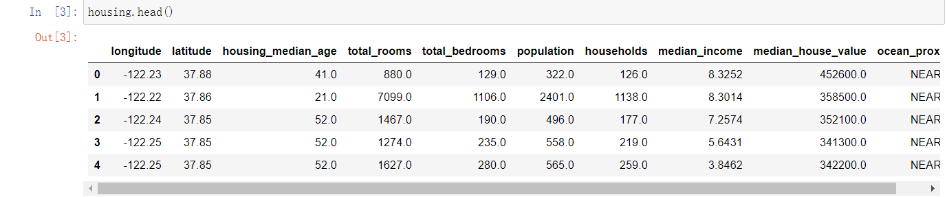
可以看出数据共有10个属性,使用info()方法可以查看属性类型及数量,describe()方法可以显示属性值摘要。
使用value_counts()方法可以查看该列又多少种分类。 1
2
3
4
5
6
7
8>>>housing['ocean_proximity'].value_counts()
output:
<1H OCEAN 9136
INLAND 6551
NEAR OCEAN 2658
NEAR BAY 2290
ISLAND 5
Name: ocean_proximity, dtype: int64
使用matplotlib库可以快速绘制直方图 1
2
3import matplotlib.pyplot as plt
housing.hist(bins = 50,figsize=(20,15))
plt.show()
快速查看数据的方法
1 | housing.head() # 前5行 |
在浏览完数据后,就需要划分训练集和测试集。在数量庞大的情况下可以选择随机划分,为保证每次运行的训练集和测试集相同,最好是分完就保存或者设定一个随机数种子。
另一个方法是更具标识符来划分,这样新增的数据可以通过打标识来解决,而前面的不需要变化。常用的标识符是哈希值。
以上讨论的都是随机划分,但有时候这样做选出来的数据不够典型。以房价为例,房价和人居收入必然是紧密联系的,我们应当在各个收入阶层都选出按照原数据比例选出。
为此我们不妨新增一个属性,起名叫“income_cat”,将人群按收入高低划分为5类
1
2
3
import numpy as np
housing["income_cat"] = np.ceil(housing["median_income"]/1.5)
housing["income_cat"].where(housing["income_cat"]<5,5.0,inplace=True)
使用Split类进行分层抽样
1 | from sklearn.model_selection import StratifiedShuffleSplit |
参数n_splits 是将训练数据分成train/test对的组数。
参数test_size和train_size是用来设置train/test对中train和test所占的比例。
参数random_state控制随机。
使用下面命令查看是否根据收入比例分配 1
2housing["income_cat"].value_counts()/len(housing)
strat_train_set["income_cat"].value_counts()/len(strat_train_set)1
2for set in (strat_train_set,strat_test_set):
set.drop(["income_cat"],axis=1,inplace=True)
2.3 从数据探索和可视化中获得洞见
分配好训练集和测试集后,我们需要对数据有更深入的洞察,先创建一个训练集副本
1
housing = strat_train_set.copy()
1
2
3
4
5housing.plot(kind="scatter",x="longitude",y="latitude",alpha=0.4,
s=housing["population"]/100,label="population",
c="median_house_value",cmap=plt.get_cmap("jet"),colorbar=True,
)
plt.legend()
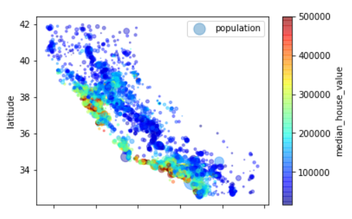
可以看出,靠近西海岸的房价会比较高。
由于数据集不大,可以使用corr()方法计算出属性间的相关性 1
2
3
4
5
6
7
8
9
10
11
12
13corr_matrix = housing.corr()
corr_matrix["median_house_value"].sort_values(ascending=False)
coutput:
median_house_value 1.000000
median_income 0.687151
total_rooms 0.135140
housing_median_age 0.114146
households 0.064590
total_bedrooms 0.047781
population -0.026882
longitude -0.047466
latitude -0.142673
Name: median_house_value, dtype: float64
试验不同属性的组合。在获得数据的相关性后,我们也可以自行构建数据,比如“房间总数”没什么用,但它除以“家庭户数”就可以得到平均一家有多少房间,同样“卧室总数”也可以这么处理。
1 | housing["rooms_per_household"] = housing["total_rooms"]/housing["households"] |
再处理完后可以再参看一次相关性 1
2
3
4
5
6
7
8
9
10
11
12
13
14output:
median_house_value 1.000000
median_income 0.687151
rooms_per_household 0.146255
total_rooms 0.135140
housing_median_age 0.114146
households 0.064590
total_bedrooms 0.047781
population_per_household -0.021991
population -0.026882
longitude -0.047466
latitude -0.142673
bedrooms_per_room -0.259952
Name: median_house_value, dtype: float64
看起来结果还可以,到了这一步我希望能将我的工作保存一下,当后面对数据进行一些处理后,我还能把这个自己组合出来的数据算出来。为此我应该建立一个函数或者是类。恰好scikit-learn已经提供了一些基础类型,只需要调用TransformerMixin和BaseEstimator作为基类,然后创建fit和transform方法。就可以将这一过程变为自定义转换器。
1 | from sklearn.base import BaseEstimator,TransformerMixin |
其中np.c_是按列合并array
2.4 机器学习算法的数据准备
这一步需要我们对数据开始正式处理,前面的都只是在观察,先回到一个干净的数据集,drop()方法会创建一个副本,不会影响到训练集。
1
2housing = strat_train_set.drop("median_house_value",axis=1)
housing_labels = strat_train_set["median_house_value"].copy()
2.4.1 数值处理
下一步就是数据清理,因为有限属性存在部分数据缺失,解决方法有三种 1. 放弃该行数据 2. 放弃该列数据 3. 补全该数据
放弃改行可以使用housing.dropna(subset=["total_bedrooms"])
放弃该列可以使用housing.drop("toatl_bedrooms",axis=1)
补全可以使用中位数、平均值、或直接用0进行补全
housing["total_bedrooms"].fillna(median)
对于补全scikit-learn还提供了imputer类来辅助处理。
这里版本问题,代码和书上略有不同 1
2
3
4from sklearn.impute import SimpleImputer
imputer = SimpleImputer(strategy="median")
housing_num = housing.drop("ocean_proximity",axis=1) # 把文本属性的先去除
imputer.fit(housing_num) # 计算出所有拟补全数据imputer.statistics_参看各列的拟补全数据。
现在可以补全数据并加回文本属性数据 1
2X = imputer.transform(housing_num)
housing_tr = pd.DataFrame(X,columns=housing_num.columns)
2.4.2 文本处理
现在完成了数据的补全,但对于文本信息我们还没进行处理,计算机对于数字更敏感,所以我们最好把文本信息转换为数字。
scikit-learn中的LabelEncoder刚好可以处理这个问题: 1
2
3
4from sklearn.preprocessing import LabelEncoder
encoder = LabelEncoder()
housing_cat = housing["ocean_proximity"]
housing_cat_encoded = encoder.fit_transform(housing_cat)
使用encoder.classes_查看映射
但这种直接的编码方法不是很好,比如海岛和近海的属性比较像,但数值却一个为0一个为4,为解决这个方法,我们可以使用OneHotEncoder进行独热编码,
1 | from sklearn.preprocessing import OneHotEncoder |
reshape(-1,1)中的-1指未设定行数,程序自动分配。
使用LabelBinarizer可以直接一步到位 1
2
3
4from sklearn.preprocessing import LabelBinarizer
encoder = LabelBinarizer(sparse_output=True)
housing_cat_1hot= encoder.fit_transform(housing_cat)
housing_cat_1hot
清洗好数据之后,我们可以利用之前编写的类将自定义的属性添加进来。
2.4.3 特征缩放
特征缩放也是数据处理中的重要一环,如果有部分数据数值过大,很有可能会影响到结果,最好是参数范围差不多。
常用缩放方法有两种: 1. 最小-最大放缩
这种方法又称为归一化,是将数据映射为0-1之间。实现方法是(目标值-最小值)/(最大值-最小值)标准化
标准化的均值总是为0,计算方法是(m-mean)/方差,它受异常值的影响会笔记小。
2.4.4 转换流水线
在数据清洗和处理的过程都是按照一个顺序进行的,很像工厂里的流水线,scikit-learn正好提供了Pipeline来支持这样的处理。
1 | from sklearn.pipeline import Pipeline |
这时候不妨回头看一下这些过程,第一个是补全,使用的SimpleImputer类,第二个是自定义的CombinedAttributesAdder类,第三个是标准化缩放类StandardScaler
它们都被要求有fit_transform()方法。考虑到scikit-learn不支持DataFrame,为此我们可能会需要用到一个df转ndarray的类。
1 | from sklearn.base import BaseEstimator, TransformerMixin |
然后把处理文本的流水线也加进来,额外的使用一个ColumnTransformer类来并行处理这些数据
1 | from sklearn.compose import ColumnTransformer |
2.5 选择和训练模型
2.5.1 建立模型
目前我们已经可以自动化洗数据了,接下来我们应该整一个回归模型!
先来个线性回归看看 1
2
3
4from sklearn.linear_model import LinearRegression
lin_reg = LinearRegression()
lin_reg.fit(housing_prepared, housing_labels)
1 | from sklearn.metrics import mean_squared_error |
emmm,貌似效果不太行,要不换成决策树? 1
2
3
4
5
6
7
8
9
10from sklearn.tree import DecisionTreeRegressor
tree_reg = DecisionTreeRegressor()
tree_reg.fit(housing_prepared, housing_labels)
housing_predictions = tree_reg.predict(housing_prepared)
tree_mse = mean_squared_error(housing_labels, housing_predictions)
tree_rmse = np.sqrt(tree_mse)
tree_rmse
output:
0.0
2.5.2 交叉验证
注意,这时候我们还没有动测试集,我们也不应该动。评估决策树模型还可以使用交叉验证,以下是k-折交叉验证的方法:
1 | from sklearn.model_selection import cross_val_score |
和线性回归做个对比
1 | lin_scores = cross_val_score(lin_reg,housing_prepared,housing_labels,scoring='neg_mean_squared_error',cv=10) |
两者半斤八两。
再来试试随机森林 1
2
3
4
5
6
7
8
9
10
11
12
13
14
15
16
17
18from sklearn.ensemble import RandomForestRegressor
forest_reg = RandomForestRegressor()
forest_reg.fit(housing_prepared, housing_labels)
housing_predictions = forest_reg.predict(housing_prepared)
forest_rmse = np.sqrt(mean_squared_error(housing_labels, housing_predictions))
forest_rmse
forest_rmse_scores = cross_val_score(forest_reg,housing_prepared,housing_labels,scoring='neg_mean_squared_error',cv=10)
forest_rmse_scores = np.sqrt(-forest_rmse_scores)
display_scrores(forest_rmse_scores)
output:
scores: [51437.73602527 49070.23768941 46719.25099192 52092.63291424
47390.46029858 51348.37861955 52067.85418266 49650.99947482
48476.17361121 54240.18337563]
Mean: 50249.39071832983
standard dviation: 2253.416487488719
略好一筹。
2.5.2 保存模型
尝试过的模型应该好好保存,因为你永远不知道哪个模型是最好的。记得还得保存一下训练参数,joblib就用来是保存的库
1 | import joblib |
2.6 微调模型
微调的一种方法是网格搜索,它会尝试多个超参数的值来找到最佳的组合,这里简单看一下即可。
1 | from sklearn.model_selection import GridSearchCV |
neg_mean_squared_error 是负均方根